
Musing
I learned differential geometry in grad school as part of learning Einstein’s theory of General Relativity. By the time I got to learning differential geometry, I had already taken courses in (flat, Euclidean) geometry, 3-D vector calculus (divergence, curl, line integrals, surface integrals, etc.), and linear algebra, so my main focus was trying to understand “what is a tensor?” (which, in my mind, was always just some collection of numbers like the components of a matrix). I thought, since I knew what a vector was, all that remained was to know what a 2-index tensor was (e.g. ) and I’d be set. This view not only made it harder for me to understand the concepts, but it also obscured the beauty of the underlying geometry.
I think the best way to learn differential geometry is actually to learn it pictorially and in a visualizable way. Descartes’ invention of Cartesian coordinates might have made us all a bit too eager to translate geometry into algebra and blind us to the beautiful coordinate-free picture.
The study of differential geometry is the study of manifolds—a certain kind of mathematical space (set of points) endowed with certain smoothness properties. We can build manifolds from the ground up, starting with the concept of a topology on top of which we add a bunch more structure. Math is often about finding the simplest structure on top of which you can “do something useful”. A topology is the simplest structure in which one can study the global properties of shapes (connectedness, compactness, etc.) while a manifold is the simplest structure on which we can “do geometry and calculus”.
Manifolds
A. Einstein
I was too much a prisoner of the idea that our equations must fully reproduce the relations between the phenomena and the chosen coordinate system…
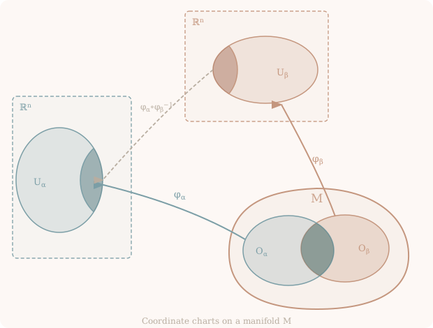
A manifold is a (smooth) topological space which “looks locally Euclidean”. What we mean precisely is that at each point of an -dimensional manifold there exists an open neighborhood which can be (smoothly, and 1-1) mapped onto an open ball , i.e. . Furthermore, given another neighborhood where and map , the maps are compatible in the intersection, i.e. (where is composition):
is 1-1, and onto. The map has component functions ; we require each to be (at least) continuous and differentiable in the usual multivariable sense, and the map as a whole to admit an inverse meeting the same conditions. The manifold is covered by these open sets with compatible maps. The collection of all maps is called an atlas. In general, we will work on manifolds where the coordinate charts are infinitely differentiable (). There is a theorem (by Whitney, sometimes called “smoothing”) that says any manifold which is at least once differentiable admits a smooth structure and that’s one reason why we just always use smooth manifolds. On occasion, we might invoke Taylor expansions and in those cases the manifold will magically turn analytic ().
Example 1
The space is itself a manifold. It can be covered trivially by a single identity map.
Example 2
The circle is a manifold. However is compact while any open subset of is not, so no single chart can cover it. Concretely, think of as the interval with endpoints identified — that identification point would have to map to two different points in if you tried to cover with a single chart.
Let it stew
This definition of a manifold seems abstract at first, but it is precisely the reason we are able to define coordinate charts () and basically do all of the normal multivariate calculus we are used to.
Musing
Defining coordinates on manifolds is so convenient that even Einstein had a hard time discarding the physical meaning of coordinates when formulating General Relativity. Einstein of course was not the only victim, as the Schwarzschild solution was considered truly singular at for quite some time after it was discovered. In my case, discarding the physical nature of coordinates was also a very difficult exercise. However, once the coordinate-centric view was discarded, I could finally see the beauty in the mathematics. Of course, if we ever have to calculate anything, we basically always have to come crawling back to the coordinates.
Vectors
V. Perkins
Vector! That’s me, because I commit crimes with both direction and magnitude. Oh yeah!
The manifold is the playground in which differential geometry lives. Vectors, forms and tensors are the objects that fill the playground.
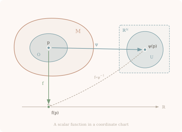
Perhaps it makes sense to start from the most basic object that can exist on a manifold: a scalar function. A (real) scalar function simply maps each point of the manifold to a real number. To keep things simple, we will ignore complex (ha!) functions for now. Because our manifold is covered by an atlas, in any open neighborhood we may define , and we may stitch all of these patches together to get an ordinary function that we are familiar with from multivariate calculus. Again, in full analogy with the coordinate map case, we can immediately lift the definitions of continuity, differentiability and analyticity from multivariate calculus. To be explicit, the function is said to be if all composition functions are at least , for every chart in the atlas.
Vectors, as the quote from the honorable V. Perkins suggests, are objects with both direction and magnitude and we think of them intuitively as “little arrows in space”. It’s nice to have intuitive pictures; however, we do have to be a little careful. In flat Euclidean space, vectors “live inside” the manifold (more precisely: the tangent space at any point is isomorphic to the base manifold) and in standard vector calculus we view them as simply an n-tuple of numbers—exactly the same way that we think of . Vectors at different points in a flat Euclidean space can be trivially compared with one another and we have an intuition for this. However, once we move to curved manifolds, vectors no longer “live inside” the manifold itself, but within the tangent space. Vectors are more intuitively thought of, in this picture, as arrows attached to a certain point in the manifold and tangent to the manifold. See fig 1.
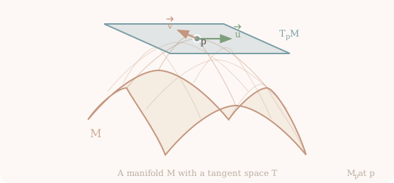
Time to get a bit more rigorous. Abstractly, we will define a tangent space as a set (of vectors) that follows the axioms of a vector space. Hence, we are free to look at vectors in any number of (equivalent) ways as long as the resulting structure forms a vector space. There are several equivalent ways to define vectors, as equivalence classes of curves, as directional derivatives, or, as we shall do here, algebraically as derivations at a point. Derivations act on the space of scalar functions: (where is the infinite dimensional space of functions on ) and obey the following two properties:
- Linearity: for and
- Leibniz:
To define vectors, we restrict ourselves to an arbitrary point so that vectors are derivations at that point (i.e. in property 2 above, remember to evaluate the resulting at the point ). The restriction to a point is important because it is only at a point that a tangent space of vectors () can be defined. Different points on a manifold have different tangent spaces. Vectors thus map functions to the real numbers, i.e. . Two vectors can be added together simply by considering their action on a test function: and properties of a vector space are satisfied trivially, e.g. distributivity of scalar multiplication:
The only non-trivial thing we have to show is that the space of derivations at a point forms a space of dimension on a dimensional manifold so that they can appropriately represent the tangent space (theorem 2.2.1 in Wald 1).
The dimension of the tangent space at a point is .
sketch: We will prove this by constructing a linearly independent set of basis vectors and show that of them suffices.
proof: First a few definitions. Let be a vector at point . Let be a function on . Let be a chart where , an open ball in , and .
Finally, for define by:
Note that is a map from . Aside: this means we can use ordinary multivariable calculus to complete the rest of the proof.
We will require a Lemma (Hadamard’s) to complete our proof (and we will prove this lemma in a separate section below). Given we have:
For some functions where:
Aside: The fact that is reused in the above 2 equations is intentional — they are the same point in .
Now we substitute , , :
Here we use the notation to mean “get the -th component of” (simply to avoid writing something like which could be confusing).
We simplify the above expression to:
Next, we apply onto the expression — note that everything in the expression are scalar functions on evaluated at some points.
is a fixed constant (it is just the value of the function at the point ) while the point varies just as varies. Recall that is a derivation (at ), therefore:
Where we have defined . Given we are able to express an arbitrary with our given basis we have proved the result.
Hadamard's Lemma
The concrete thing we need to prove are two formulas from the above theorem:
Everything we do here is just “standard (multi-variate) calculus”. We start with the 1-D case as a warm up. We have the fundamental theorem of calculus (in suggestive form) for a single variable:
and we make the substitution so that when and :
Now we imagine that we are taking a line integral from some initial point to an end point along some curve such that and in :
Let me explain the notation shift here real quick. The left hand side of the above expression is likely the line integral we are familiar with from standard multivariable calculus. Since it will be awkward to maintain the vector notation in this lemma, we will write it instead in component form that you see on the right hand side. You can already see some sneakiness in the notation here. Why does have components with the downstairs? This is in anticipation of the fact that actually the thing we need is a gradient, which is naturally a one-form (explained later) and a one form’s components have indices downstairs. The equation presented is just to help you think about a line integral. This Lemma is too long already, so I’m going to stop expositing here.
Next, let’s assume that the vector field that we think about in that line integral comes from a conservative one where for some function . Then the integral will only depend on the start and end points given by the gradient theorem:
What remains is to plug in the components of into , note that and turn the integral into a definite integral in 1-D:
Since the integral doesn’t really care about the curve except for at the end points, we can just take the simple curve where simply forms a straight line from to : so that: . We plug this directly back to get:
We plug in the expression we had for to get finally:
Where we have defined and we can see:
Musing
In general we won’t do too much theorem proving in the nerd nook. I only presented this one here because in Wald 1, part of the above is given as a homework assignment. So you basically just watched me do self-assigned homework lol.
One-Forms
Having defined vectors at a point , it is simple to define the one-forms at the same point as the set of linear maps taking vectors to the real numbers: equipped with addition ( are one-forms and is a vector) and scalar multiplication ( is a real number). One-forms live in the cotangent space . We can now immediately define, via symmetry, the action of vectors on one forms , where , so that vectors are linear maps of one-forms to real numbers. For clarity, what we mean by linearity is the following:
Where and . The reason we call these objects “one-forms” will be made clear in the next section. The cotangent space is itself a vector space which can be easily checked given the above definitions.
Warning
If you call one-forms vectors because they are elements of a vector space then you will get coal in your stockings for Christmas.
The spaces and are isomorphic (as vector spaces) to each other and are called “dual”. However, without a metric (which we get to eventually below) there is not a unique natural isomorphism between the two spaces. Nevertheless, a basis on does pick out a naturally dual basis on (and vice-versa) via the requirement where is the “Kronecker-Delta” symbol which is equal to when and otherwise. We pretty much will always use naturally dual bases since they make pretty much all calculations easier.
There is an object in elementary vector calculus which is naturally a one-form. This is the gradient of a function, which we often see as .
Tensors, n-forms, wedge products and grassman algebra, fields, lie derivative, exterior derivative, Stokes' theorem, Frobenius' theorem, fiber bundles, connections, metric, curvature, symplectic manifolds, homotopy